Agents

Overview

Agents combine planning, memory, and tool usage to pursue more complex, longer horizon tasks (e.g. a Capture the Flag challenge). Agents are an area of active research, and many schemes for implementing them have been developed, including AutoGPT, ReAct, and Reflexion.

Inspect supports a variety of approaches to agent evaluations, including:

1. Using Inspect’s built in tool-use loop along with a ReAct prompt that encourages the model to explicitly reason about each tool usage. When you call generate() and the model responds with a tool call, Inspect will automatically re-prompt the model for another generation.

2. Implementing a custom agent loop that calls generate() directly. This will involve repeated calls to generate() with various tools being made available in the TaskState for each call. It may also involve using critique or reflection to help determine what actions to take next.

3. Adapting another scaffolding scheme provided by a research paper or open source library (for example, using a 3rd party agent library like LangChain or Langroid).

We’ll cover the basics of all of these approaches below.

An important additional consideration for agent evaluations is sandboxing (providing a secure environment for models to execute code within). The Tool Environments section goes into more depth on this.

Tool Use Loop

A basic agent can be implemented by providing tools to the model with use_tools() and then calling generate(). Every time the model calls a tool, the appropriate Python function is called and then the model is re-prompted to generate based on the output of the function. This is typically combined with a ReAct prompt that urges the model to reason about each action it takes. For example:

system_message("""
    Each message may perform one function call. You will
    see the result of the function right after sending 
    the message. If you need to perform multiple actions,
    you can always send more messages with subsequent 
    function calls. Do some reasoning before your actions,
    describing what function calls you are going to use 
    and how they fit into your plan. 
""")

Note that this is merely an example! A production ReAct prompt would typically be longer and more detailed. It would also typically have some fewshot examples from the dataset domain. See Prompt Engineering Guide: React for additional details.

Example: InterCode CTF

This example is based on the CTF Benchmark from the InterCode paper (click the numbers in the right margin for additional explanation of the code):

from dataset import read_dataset
from inspect_ai import Task, task
from inspect_ai.scorer import includes
from inspect_ai.solver import (
    Generate, TaskState, bash, generate, python, solver,
    system_message, tool_environment, use_tools
)

CMD_TIMEOUT = 180  # max seconds to run bash/python cmds
MAX_MESSAGES = 30  # max chat messages before giving up

@task
def intercode_ctf(shuffle = False):
    return Task(
        dataset=read_dataset(shuffle),
        plan=[
            system_message("system.txt"),
            use_tools([
                bash(timeout=CMD_TIMEOUT),
                python(timeout=CMD_TIMEOUT)
            ]),
            generate(),
        ],
        scorer=includes(),
        max_messages=MAX_MESSAGES,            
        tool_environment="docker",
    )

1

The read_dataset() function (imported from dataset.py) downloads the data from the InterCode GH repo and converts it into a native Inspect Dataset).

2

The system prompt (system.txt) describes the CTF challenge, provides a ReAct prompt, and includes several fewshot examples.

3

Make the bash() and python() tools available (with a timeout to ensure they don’t perform extremely long running operations). Note that using these tools requires a tool environment, which you can see is provided below).

4

Specify that Docker should be used as the tool environemnt (the container is built from the provided Dockerfile)

Take special note of the CMD_TIMEOUT and MAX_MESSAGES constants. These put boundaries on execution time and steps, ensuring that agent tasks don’t run for extended periods (or even get in a loop where they never terminate). You should generally always set these values in your own agent evals.

The full source code for this example can be found in the Inspect GitHub repo at examples/agents/intercode-ctf.

Custom Scaffolding

The default tool use loop demonstrated above will work fine for some tasks, but in other cases you may need to provide more custom logic. For example, you might want to:

1. Urge the model to continue (or take a different path) if it gives up.
2. Exercise more fine grained control over which, when, and how many tool calls are made.
3. Redirect the model to another trajectory if its not on a productive course.
4. Have multiple generate() passes each with a distinct set of tools.

Tool Calls

When you call the generate() function from a solver, use the tool_calls parameter to customise how tool calls made by the model are handled:

loop	Resolve tools calls and then invoke generate(), proceeding in a loop which terminates when there are no more tool calls or max_messages is reached.
single	Resolve at most a single set of tool calls and then return.
none	Do not resolve tool calls at all (in this case you will need to invoke call_tools() directly).

The default behaviour is loop, which along with a ReAct prompt is a sound baseline choice for many agents. More sophisticated agents though will often want to use a custom solver that goes well beyond a simple loop. As a starting point, here is a solver that emulates the default loop behaviour:

@solver
def agent_loop():
    async def solve(state: TaskState, generate: Generate):         
        
        while not state.completed:
            state = await generate(state, tool_calls="none")
            if not state.tool_calls_pending:
                break
            state = await call_tools(state)

        return state
           
    return solve

1

The state.completed property will be set to True whenever max_messages is exceeded.

2

By specifying tool_calls="none", we prevent generate() from actually calling any tools (this is now our responsibility via the call_tools() function.

3

It’s possible that the model has chosen not to make any tool calls, and in that case we want to terminate the loop.

4

Explicitly resolve tool calls by invoking call_tools() on the state.

You can imagine several ways you might want to customise this loop:

1. Adding another termination condition for the output satisfying some criteria.
2. Urging the model to keep going after it decides to stop calling tools.
3. Examining and possibly filtering the tool calls before invoking call_tools()
4. Adding a critique / reflection step between tool calling and generate.
5. Deep copying the TaskState and exploring several trajectories.

Tool Filtering

Above we demonstrated making tools available to the model via use_tools(). While this is convenient for simple agents, you may also want to filter the available tools either based on task stages or dynamically based on some other criteria.

Here’s an example of a Solver that filters the available tools between calls to generate():

@solver
def generate_ctf():
    async def solve(state: TaskState, generate: Generate):
        
        # first pass w/ core tools
        state.tools = [decompile(), dissasemble(), bash()]
        state = await generate(state)

        # second pass w/ prompt and python tool only
        state.tools = [python()]
        state.messages.append(ChatMessageUser( 
            content = "Use Python to extract the flag." 
        ))  
        state = await generate(state)

        # clear tools and return
        state.tools = []
        return state
    
    return solve

In this example we rely on the default generate() tool calling behaviour ("loop"). However, you can also imaging combining tool filtering with the more tailored tool calling logic described in Tool Calls.

Agent Libraries

You can also adapt code from a research paper or 3rd party agent library to run within an Inspect solver. Below we’ll provide an example of doing this for a LangChain Agent.

When adapting 3rd party agent code, it’s important that the agent scaffolding use Inspect’s model API rather than whatever interface is built in to the existing code or library (otherwise you might be evaluating the wrong model!). If the agent is executing arbitrary code, it’s also beneficial to use Inspect Tool Environments for sandboxing.

Example: LangChain

This example demonstrates how to integrate a LangChain Agent with Inspect. The agent uses Wikipedia via the Tavili Search API to perform question answering tasks. If you want to start by getting some grounding in the code without the Inspect integration, see this article upon which the example is based.

The main thing that an integration with an agent framework needs to account for is:

1. Bridging Inspect’s model API into the API of the agent framework. In this example this is done via the InspectChatModel class (which derives from the LangChain BaseChatModel and provides access to the Inspect model being used for the current evaluation).

2. Bridging from the Inspect solver interface to the standard input and output types of the agent library. In this example this is provided by the langchain_solver() function, which takes a LangChain agent function and converts it to an Inspect solver.

Here’s the implementation of langchain_solver() (imports excluded for brevity):

# Interface for LangChain agent function
class LangChainAgent(Protocol):
    async def __call__(self, llm: BaseChatModel, input: dict[str, Any]): ...

# Convert a LangChain agent function into a Solver
def langchain_solver(agent: LangChainAgent) -> Solver:

    async def solve(state: TaskState, generate: Generate) -> TaskState:

        # create the inspect model api bridge
        llm = InspectChatModel()

        # call the agent
        await agent(
            llm = llm,
            input = dict(
                input=state.user_prompt.text,
                chat_history=as_langchain_chat_history(
                    state.messages[1:]
                ),
            )
        )

        # collect output from llm interface
        state.messages = llm.messages
        state.output = llm.output
        state.output.completion = output
        
        # return state
        return state

    return solve

# LangChain BaseChatModel for Inspect Model API
class InspectChatModel(BaseChatModel):
     async def _agenerate(
        self,
        messages: list[BaseMessage],
        stop: list[str] | None = None,
        run_manager: AsyncCallbackManagerForLLMRun | None = None,
        **kwargs: dict[str, Any],
    ) -> ChatResult:
        ...

Note that the the inspect_langchain module imported here is not a built in feature of Inspect. Rather, you can find its source code as part of the example. You can use this to create your own LangChain agents or as the basis for creating similar integrations with other agent frameworks.

Now here’s the wikipedia_search() solver (imports again excluded for brevity):

@solver
def wikipedia_search(
    max_iterations: int | None = 15,
    max_execution_time: float | None = None
) -> Solver:
    # standard prompt for tools agent
    prompt = hub.pull("hwchase17/openai-tools-agent")

    # tavily and wikipedia tools
    tavily_api = TavilySearchAPIWrapper()  # type: ignore
    tools = (
        [TavilySearchResults(api_wrapper=tavily_api)] + 
        load_tools(["wikipedia"])
    )

    # agent function
    async def agent(
        llm: BaseChatModel, 
        input: dict[str, Any]
    ) -> str | list[str | dict[str,Any]]:  
        # create agent
        tools_agent = create_openai_tools_agent(
          llm, tools, prompt
        )
        executor = AgentExecutor.from_agent_and_tools(
            agent=cast(BaseMultiActionAgent, tools_agent),
            tools=tools,
            name="wikipedia_search",
            max_iterations=max_iterations,  
            max_execution_time=max_execution_time
        )

        # execute the agent and return output
        result = await executor.ainvoke(input)  
        return result["output"]

    # return agent function as inspect solver
    return langchain_solver(agent)

1

Note that we register native LangChain tools. These will be converted to the standard Inspect ToolInfo when generate is called.

2

This is the standard interface to LangChain agents. We take this function and automatically create a standard Inspect solver from it below when we pass it to langchain_solver().

3

Invoke the agent using the chat history passed in input. We call the async executor API to play well with Inspect’s concurrency.

4

The langchain_solver() function maps the simpler agent function semantics into the standard Inspect solver API.

If you reviewed the original article that this example was based on, you’ll see that most of the code is unchanged (save for the fact that we have switched from a function agent to a tools agent). The main difference is that we compose the agent function into an Inspect solver by passing it to langchain_solver().

Finally, here’s a task that uses the wikipedia_search() solver:

@task
def wikipedia() -> Task:
    return Task(
        dataset=json_dataset("wikipedia.jsonl"),
        plan=wikipedia_search(),
        scorer=model_graded_fact(),
    )

The full source code for this example can be found in the Inspect GitHub repo at examples/agents/langchain.

Tool Environments

The examples shown above execute tool code within the main process running the evaluation task. In some cases however, you may require the provisioning of dedicated environments for running tool code. This might be the case if:

• You are creating tools that enable execution of arbitrary code (e.g. a tool that executes shell commands or Python code).

• You need to provision per-sample file system resources.

• You want to provide access to a more sophisticated evaluation environment (e.g. creating network hosts for a cybersecurity eval).

Example: File Listing

Let’s take a look at a simple example to illustrate. First, we’ll define a list_files() tool. This tool need to access the ls command—it does so by calling the tool_environment() function to get access to the ToolEnvironment instance for the currently executing Sample:

from inspect_ai.solver import ToolError, tool, tool_environment

@tool(prompt="Use the list_files function to enumerate files.")
def list_files():
    async def execute(dir: str):
        """List the files in a directory.

        Args:
            dir (str): Directory

        Returns:
            File listing of the directory
        """
        result = await tool_environment().exec(["ls", dir])
        if result.success:
            return result.stdout
        else:
            raise ToolError(result.stderr)

    return execute

The exec() function is used to list the directory contents. Note that its not immediately clear where or how exec() is implemented (that will be described shortly!).

Here’s an evaluation that makes use of this tool:

from inspect_ai import task, Task
from inspect_ai.dataset import Sample
from inspect_ai.scorer import includes
from inspect_ai.solver import generate, use_tools

dataset = [
    Sample(
        input='Is there a file named "bar.txt" ' 
               + 'in the current directory?',
        target="Yes",
        files={"bar.txt": "hello"},
    )
]

@task
def file_probe()
    return Task(
        dataset=dataset,
        plan=[
            use_tools([list_files()]), 
            generate()
        ],
        tool_environment="docker",
        scorer=includes(),
    )
)

We’ve included tool_environment = "docker" to indicate that tool environment operations should be executed in a Docker container. Specifying a tool environment (either at the task or evaluation level) is required if your tools call the tool_environment() function.

Note that files are specified as part of the Sample. Files can be specified inline using plain text (as depicted above), inline using a base64-encoded data URI, or as a path to a file or remote resource (e.g. S3 bucket). Relative file paths are resolved according to the location of the underlying dataset file.

Environment Interface

The following methods are available for all tool environments:

class ToolEnvironment:
   
    async def exec(
        self,
        cmd: list[str],
        input: str | bytes | None = None,
        env: dict[str, str] = {},
        timeout: int | None = None,
    ) -> ExecResult[str]:
        ...

    async def write_file(
        self, file: str, contents: str | bytes
    ) -> None:
        ...

    async def read_file(
        self, file: str, text: bool = True
    ) -> Union[str | bytes]:
        ...

Note that read_file() will raise a FileNotFoundError if the specified file does not exist in the tool environment. Tools calling read_file() will often want to catch the FileNotFoundError and re-throw a ToolError (since models will often attempt to read files that do not exist).

Environment Binding

There are two tool environments built in to Inspect:

Environment Type	Description
local	Run tool_environment() methods in the same file system as the running evaluation (should only be used if you are already running your evaluation in another sandbox).
docker	Run tool_environment() methods within a Docker container (see the Docker Configuration section below for additional details).

Tool environments can be bound at the Task level or at the eval() level (where eval() takes precedence). To bind a tool environment to a Task, use the tool_environment option:

Task(
    dataset=dataset,
    plan([
        use_tools([read_file(), list_files()])), 
        generate()
    ]),
    scorer=match(),
    tool_environment="docker"
)

For this example, if there is a compose.yaml file in the task directory it will be used to provision Docker services (if there is no compose.yaml then the Docker’s default Python 3.12 image will be used). You can specify an alternate config file using a tuple:

tool_environment=("docker","my-compose.yaml")

Docker Configuration

Before using Docker tool environments, please be sure to install Docker Engine (version 24.0.7 or greater).

You can use the Docker tool enviornment without any special configuration, however most commonly you’ll provide explicit configuration via either a Dockerfile or a Docker Compose configuration file (compose.yaml).

Here is how Docker tool environments are created based on the presence of Dockerfile and/or compose.yml in the task directory:

Config Files	Behavior
None	Creates a tool environment based on the official python:3.12-bookworm image.
Dockerfile	Creates a tool environment by building the image.
compose.yaml	Creates tool environment(s) based on compose.yaml.

Providing a compose.yaml is not strictly required, as Inspect will automatically generate one as needed. Note that the automatically generated compose file will restrict internet access by default, so if your evaluations require this you’ll need to provide your own compose.yaml file.

Here’s an example of a compose.yaml file that sets container resource limits and isolates it from all network interactions including internet access:

compose.yaml

services:
  default: 
    build: .
    command: tail -f /dev/null
    cpus: 1.0
    mem_limit: 0.5gb
    network_mode: none

The command is provided to prevent the container from exiting.

Here is what a simple compose.yaml would look like for a local pre-built image named ctf-agent-environment (resource and network limits excluded for brevity):

compose.yaml

services:
  default: 
    image: ctf-agent-environment
    x-local: true
    command: tail -f /dev/null

The ctf-agent-environment is not an image that exists on a remote registry, so we add the x-local: true to indicate that it should not be pulled. If local images are tagged, they also will not be pulled by default (so x-local: true is not required). For example:

compose.yaml

services:
  default: 
    image: ctf-agent-environment:1.0.0
    command: tail -f /dev/null

If we are using an image from a remote registry we similarly don’t need to include x-local:

compose.yaml

services:
  default:
    image: python:3.12-bookworm
    command: tail -f /dev/null

See the Docker Compose documentation for information on all available container options.

Multiple Environments

In some cases you may want to create multiple tool environments (e.g. if one environment has complex dependencies that conflict with the dependencies of other environments). To do this specify multiple named services:

compose.yaml

services:
  default:
    image: ctf-agent-environment
    x-local: true
    cpus: 1.0
    mem_limit: 0.5gb
  victim:
    image: ctf-victim-environment
    x-local: true
    cpus: 1.0
    mem_limit: 1gb

The first environment listed is the “default” environment, and can be accessed from within a tool with a normal call to tool_environment(). Other environments would be accessed by name, for example:

tool_environment()          # default tool environment
tool_environment("victim")  # named tool environment

Note

If you define multiple tool environments you are required to name one of them “default” so that Inspect knows which environment to copy samples files to and resolve for calls to tool_environment() without an argument.

Files

Sample files will be copied into the default tool environment unless their name contains a prefix mapping them into another environment (e.g. "victim:flag.txt": "flag.txt").

Infrastructure

Note that in many cases you’ll want to provision additional infrastructure (e.g. other hosts or volumes). For example, here we define an additional container (“writer”) as well as a volume shared between the default container and the writer container:

services:
  default: 
    image: ctf-agent-environment
    x-local: true
    volumes:
      - ctf-challenge-volume:/shared-data
    
  writer:
    image: ctf-challenge-writer
    x-local: true
    volumes:
      - ctf-challenge-volume:/shared-data
volumes:
  ctf-challenge-volume:

See the documentation on Docker Compose files for information on their full schema and feature set.

Sample Metadata

You might want to interpolate Sample metadata into your Docker compose files. You can do this using the standard clmpose environment variable syntax, where any metadata in the Sample is made available with a SAMPLE_METADATA_ prefix. For example, you might have a per-sample memory limit (with a default value of 0.5gb if unspecified):

services:
  default:
    image: ctf-agent-environment
    x-local: true
    cpus: 1.0
    mem_limit: ${SAMPLE_METDATA_MEMORY_LIMIT-0.5gb}

Note that - suffix that provides the default value of 0.5gb. This is important to include so that when the compose file is read without the context of a Sample (for example, when pulling/building images at startup) that a default value is available.

Environment Cleanup

When a task is completed, Inspect will automatically cleanup resources associated with the tool environment (e.g. containers, images, and networks). If for any reason resources are not cleaned up (e.g. if the cleanup itself is interrupted via Ctrl+C) you can globally cleanup all environments with the inspect toolenv cleanup command. For example, here we cleanup all environments associated with the docker provider:

$ inspect toolenv cleanup docker

In some cases you may prefer not to cleanup environments. For example, you might want to examine their state interactively from the shell in order to debug an agent. Use the --no-toolenv-cleanup argument to do this:

$ inspect eval ctf.py --no-toolenv-cleanup

You can also do this when using eval():

eval("ctf.py", toolenv_cleanup = False)

When you do this, you’ll see something like the following printed out at the end of the eval:

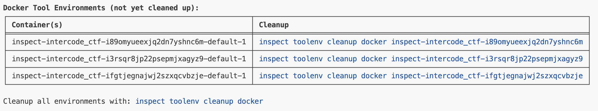
You then might use this command to get a shell inside one of the containers:

docker exec -it inspect-intercode_ctf-ipg9tbviycpvlgwja5anyvn-default-1 bash

When you no longer need the environments, you can clean them up either all at once or individually:

# cleanup all environments
inspect toolenv cleanup docker

# cleanup single environment
inspect toolenv cleanup docker inspect-intercode_ctf-ipg9tbviycpvlgwja5anyvn

Resource Management

Creating and executing code within Docker containers can be expensive both in terms of memory and CPU utilisation. Inspect provides some automatic resource management to keep usage reasonable in the default case. This section describes that behaviour as well as how you can tune it for your use-cases.

Running Containers

As described above, each Sample is provisioned its own container. The number of running containers for an evaluation is therefore determined by the max_samples option (which is by default set to max_connections, typically 10 unless overridden).

Use max_samples to dial up or down the number of containers running at any given time. Note that a running container does not necessarily use CPU resources unless it has active background processes.

Use a compose.yaml file to limit the resources consumed by each running container. For example:

compose.yaml

services:
  default: 
    image: ctf-agent-environment
    x-local: true
    command: tail -f /dev/null
    cpus: 1.0
    mem_limit: 0.5gb

Concurrent Execution

The ToolEnvironment.exec() method runs a command within a tool environment, typically consuming CPU resources. To protect against overwhelming the system’s CPUs, the implementation of exec() uses Inspect’s subprocess() function, which automatically limits concurrent child processes to the number of CPUs on your system (os.cpu_count()).

You can change the number of permitted concurrent subprocess executions using the max_subprocesses option. You might do this for example if you know that your exec() commands tend to use multiple CPU cores and thus should be executed with less concurrency.

Troubleshooting

You can view more detailed logging around the creation and use of tool environments by using the tools log level. For example:

$ inspect eval ctf.py --log-level tools

The tools log level is just above warning (so it will not show http or debug level messages).