Skewed Score Analysis

Handling ordinal data with ordered logistic models

Overview

These examples demonstrate how to analyse ordinal evaluation data with skewed distributions using ordered logistic regression models. Located in examples/skewed_score/, they showcase custom model implementations and specialised visualisations for ordinal outcomes.

This notebook implements methods from the paper: Skewed Score: A Statistical Framework to Assess Autograders

WarningNo inspect logs

We cannot provide the inspect logs for this example, just the extracted csvs.

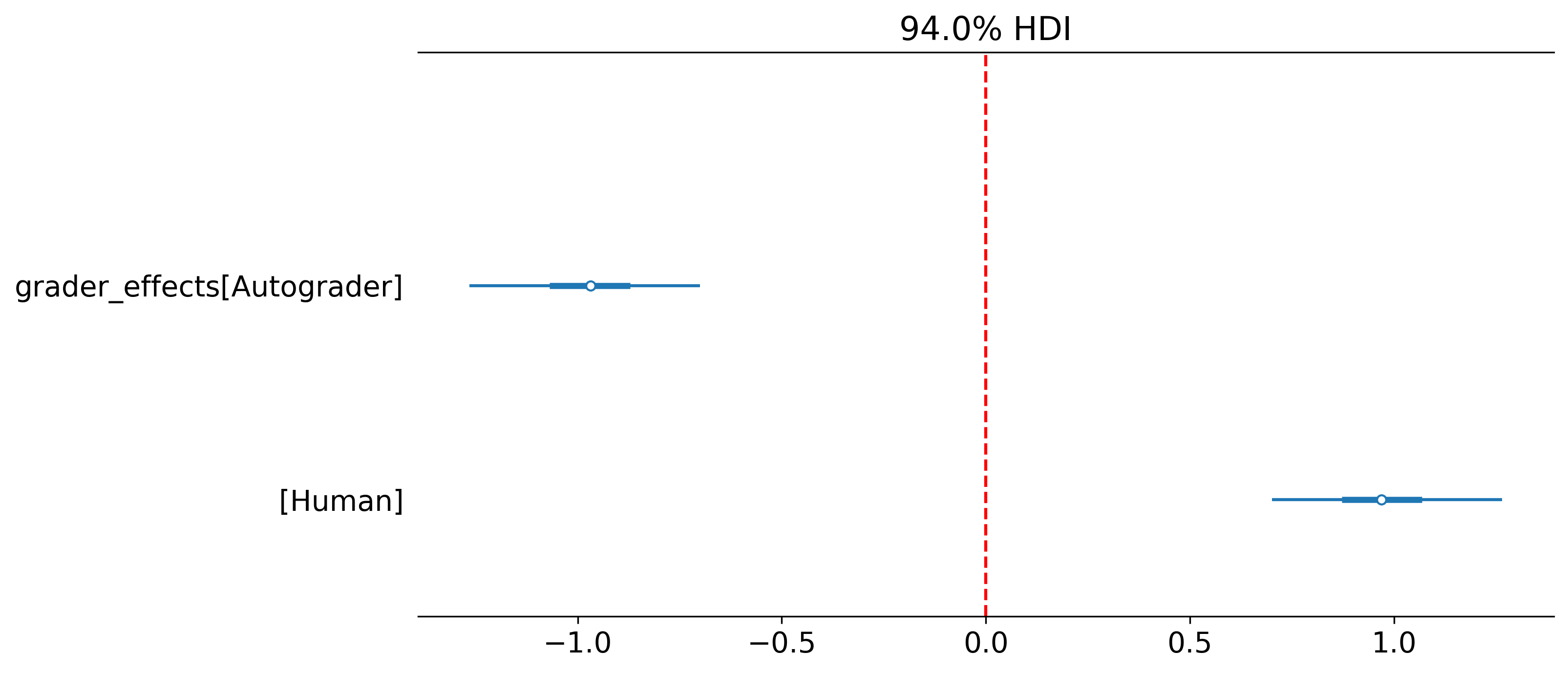
Question 1: Grader Effects Analysis

Analyses how different graders affect score distributions on a 0-10 rating scale.

Purpose

• Estimate grader-specific effects
• Account for ordinal score structure
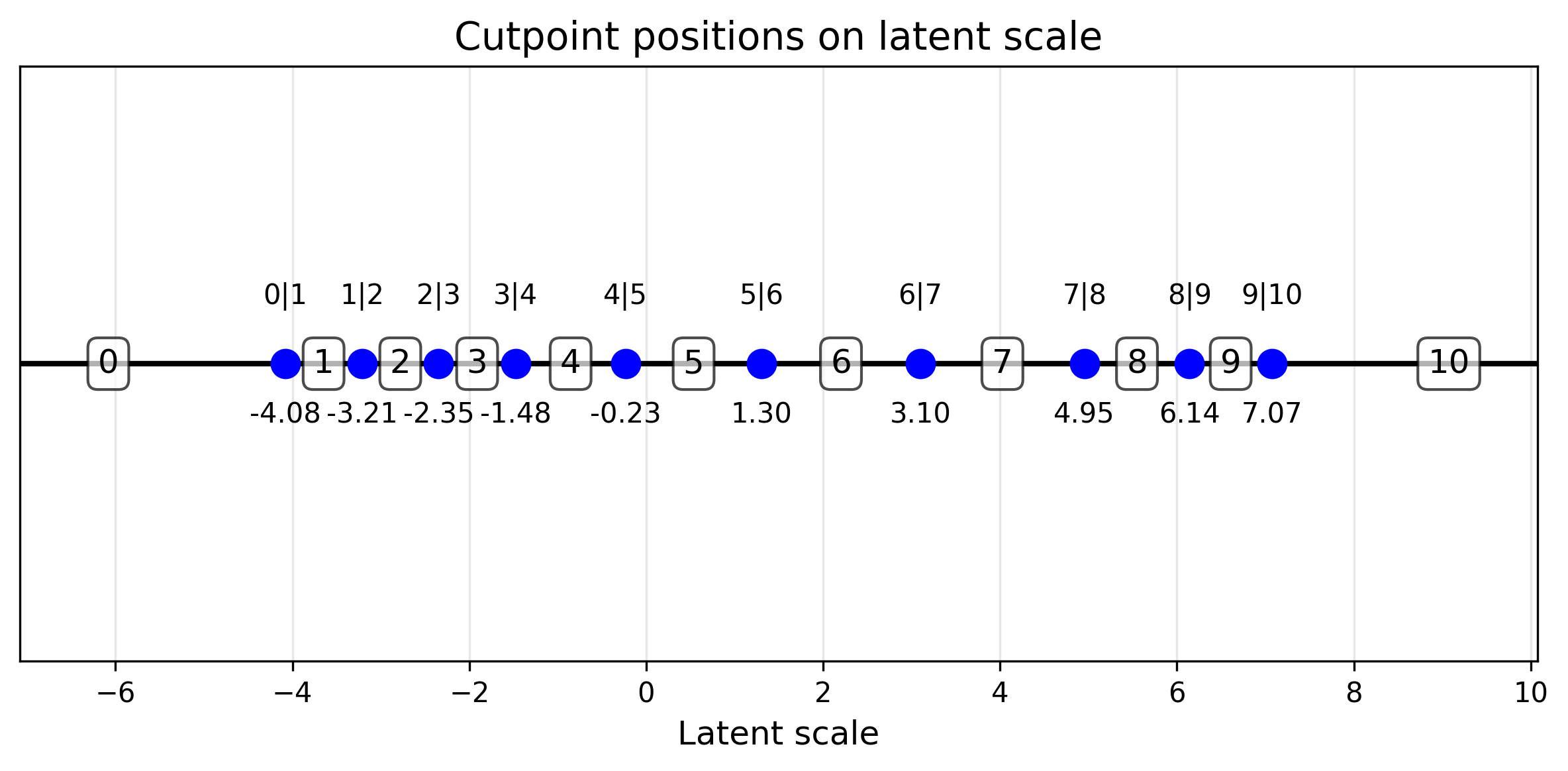
• Visualise cutpoint distributions

Configuration

data_process:
  processors:
    - extract_observed_feature: {feature_name: score}  # 0-10 rating
    - extract_features: {categorical_features: [grader], effect_coding_for_main_effects: true}

1

Here we use effect coding where parameters sum to zero, this make interpretation of the values easier.

Model Implementation

As each item awarded a score between 0 and 10, need need to use a special likelihood function. Good news HiBayES already supports this with the ordered_logistic_model model.

model:
  models:
    - name: ordered_logistic_model
      config:
        tag: version_1
        main_effects: ["grader"]
        num_classes: 11  # for 0-10 scale
        effect_coding_for_main_effects: true
        fit:
          samples: 2000
          chains: 4

1

along with the cutpoints (see below) and the global intercept we add the grader parameter to see how different graders (a human and an LLM) score.

Visualisations

A mixture of custom and default communicators are used to interpret the data

communicate:
  path: ../custom_communicators.py
  communicators:
    - cutpoint_plot
    - ordered_residuals_plot
    - category_frequency_plot
    - forest_plot: {vars: ["grader_effects"], combined: true, vertical_line: 0}

1

Specify the file which contains your custom communicators.

Here we can see the learn cutpoints along the latent scale, showing the degree of shift required to change between each ordinal score.

Here we see the standard forest plot from HiBayES, showing a significant difference between autrograder and human grades

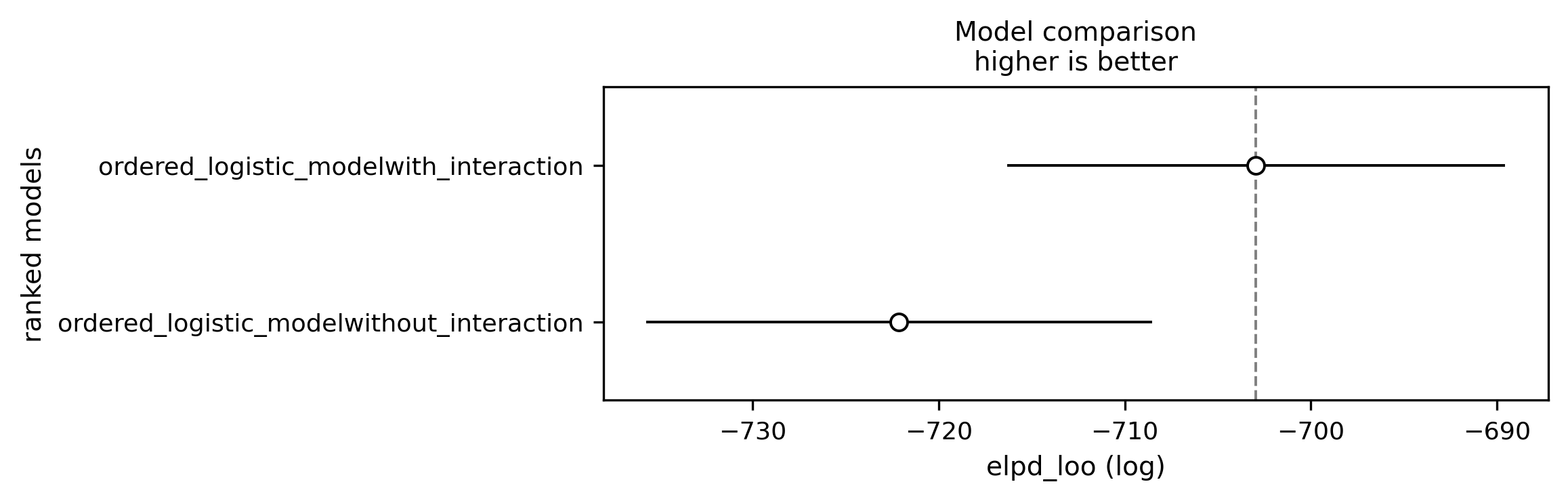
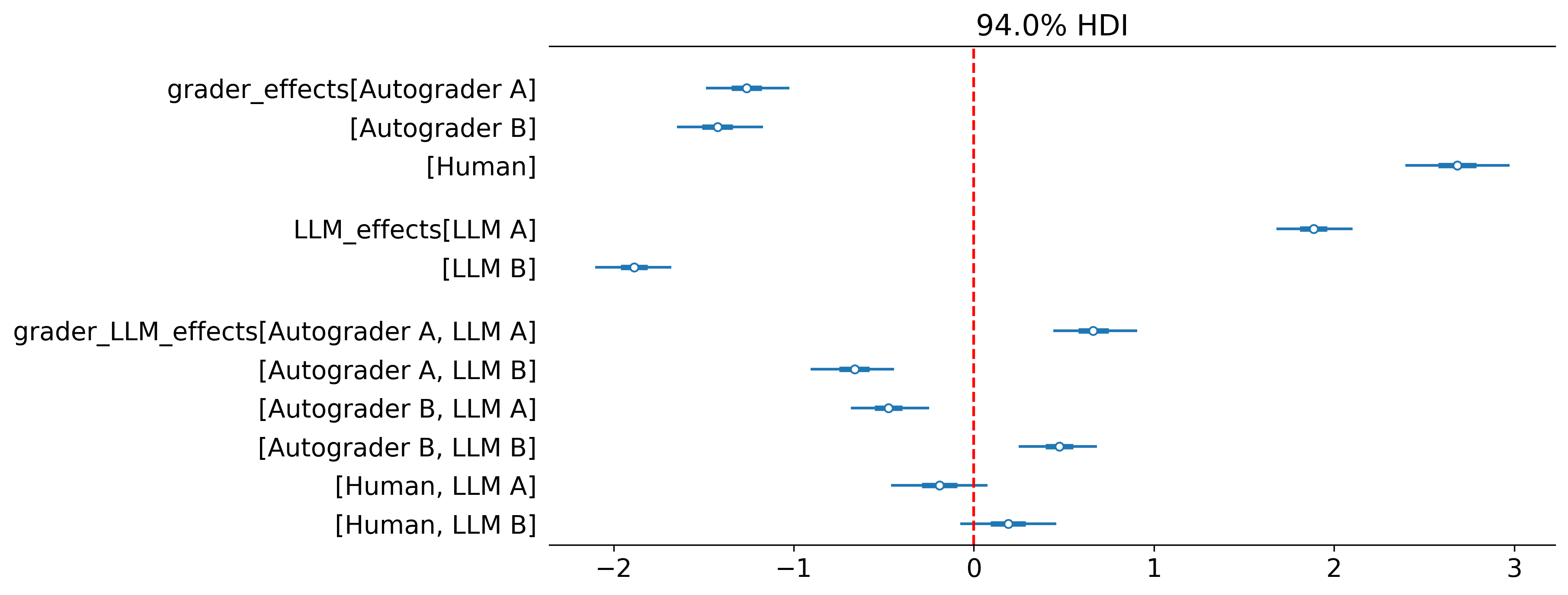
Question 2: Do autograders favour their own generation?

To do this we can add an interaction term to see if autograders favour their own generation.

model:
  models:
    - name: ordered_logistic_model
      config:
        tag: with_interaction
        main_effects: ["grader", "LLM"]
        interactions: [["grader", "LLM"]]
        num_classes: 11  # for 0-10 scale
        effect_coding_for_main_effects: true
    - name: ordered_logistic_model
      config:
        tag: without_interaction
        main_effects: ["grader", "LLM"]
        num_classes: 11
        effect_coding_for_main_effects: true

check:
  checkers:
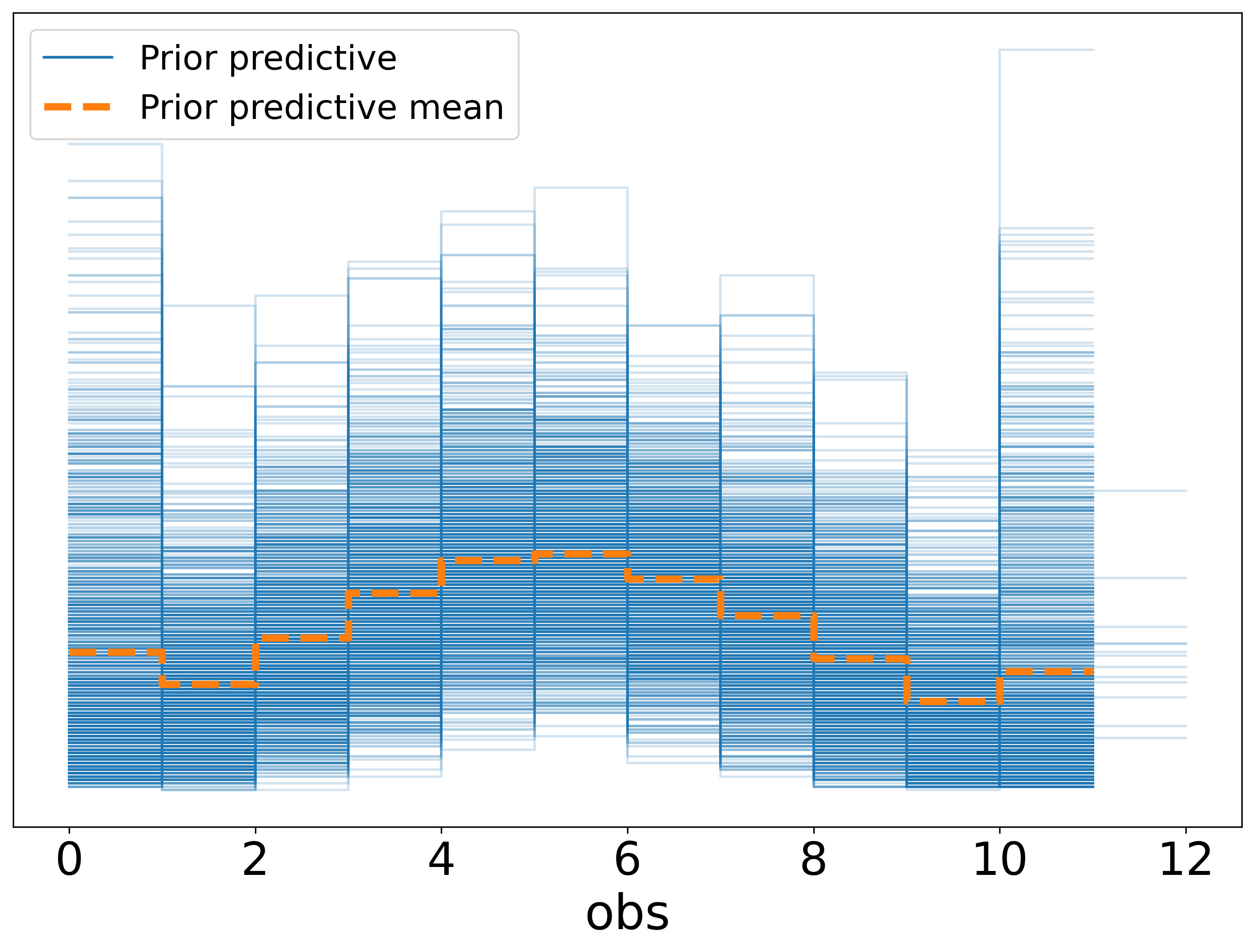
    - prior_predictive_plot: {interactive: false}
    - divergences
    - r_hat
    - ess_bulk
    - ess_tail
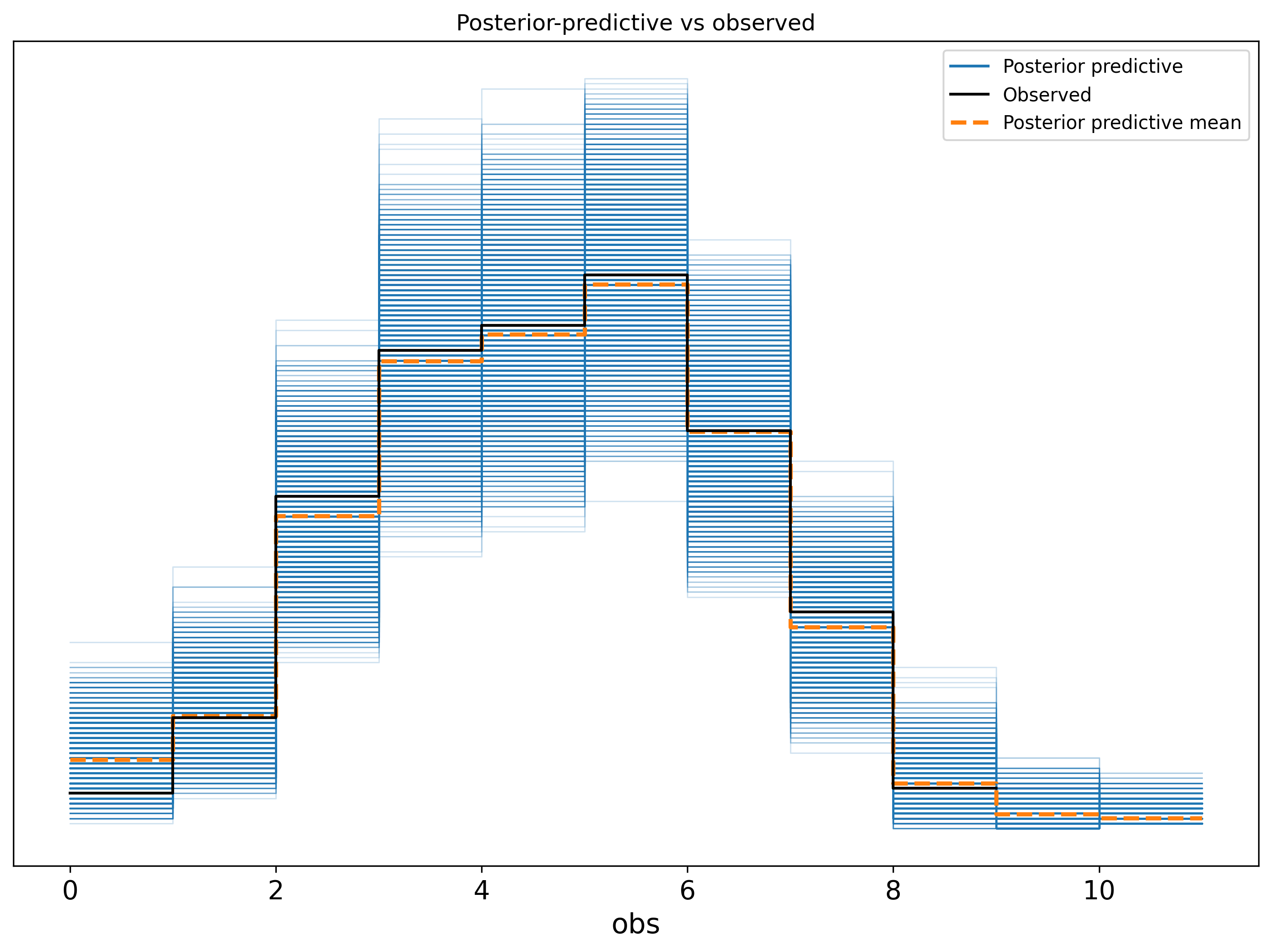
    - posterior_predictive_plot: {interactive: false}
    - waic

1

Here is where we add the interaction!

2

It is still important to assess the fit of a model without an interaction. Maybe it is a better fit and you will find no evidence to suggest autograders favour their own generations.

3

we are showing the checker config here as when there are lots of models to fit having to online approve the prior and posterior predictive checks can become quite buredomsome. Here we have turned off the interactive element and you can review the checks offline. See the plots below.

Here we sample from the model before it has been trained on any data. Are the assumptions good?

Here we sample from the model after it has been fitted. Is it a good fit?

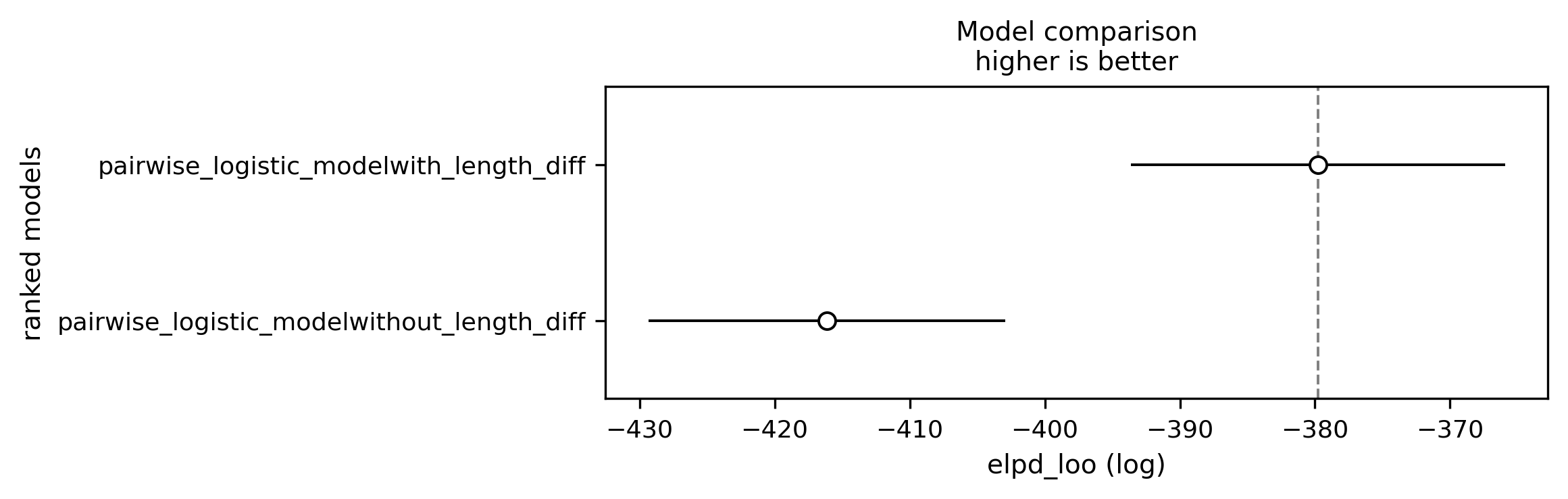
For the comparison the model_comparison_plot was added to the communicators.

When we add the interaction the model predicts the data better

Whats more, the autograder A x LLM A and autograder B x LLM B are significantly not zero suggesting preference!!

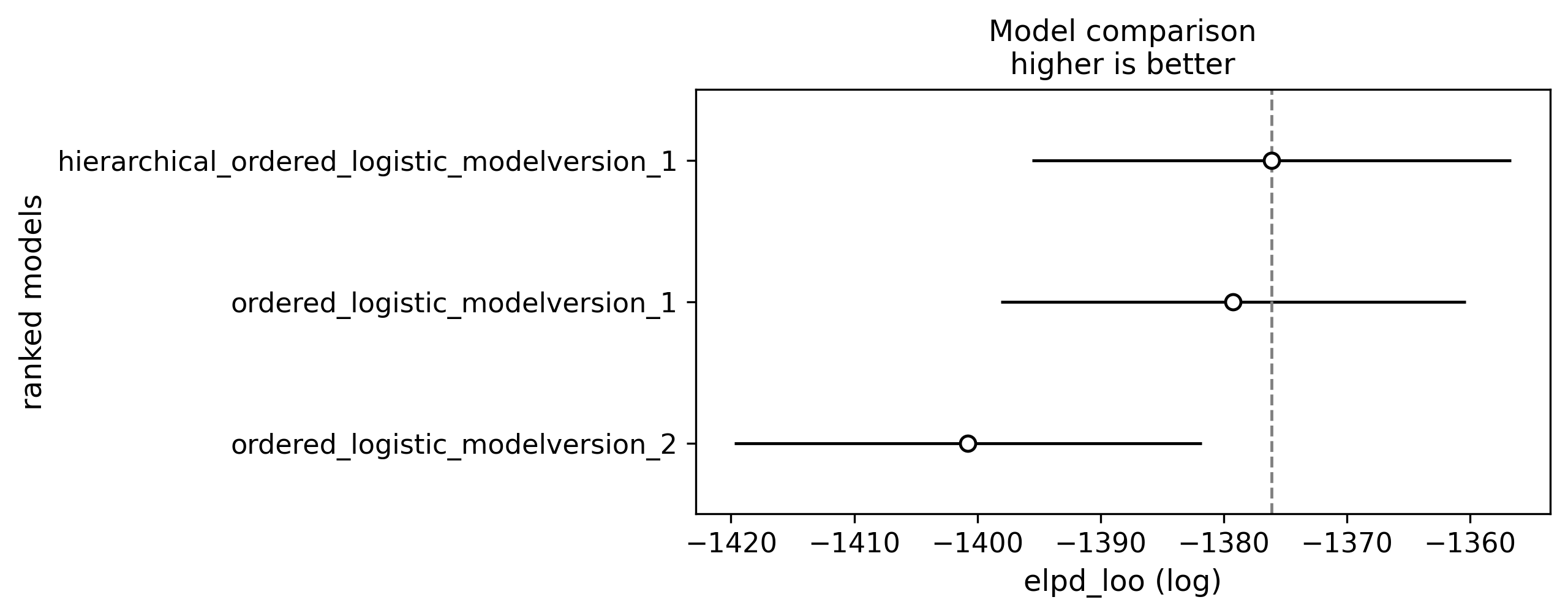
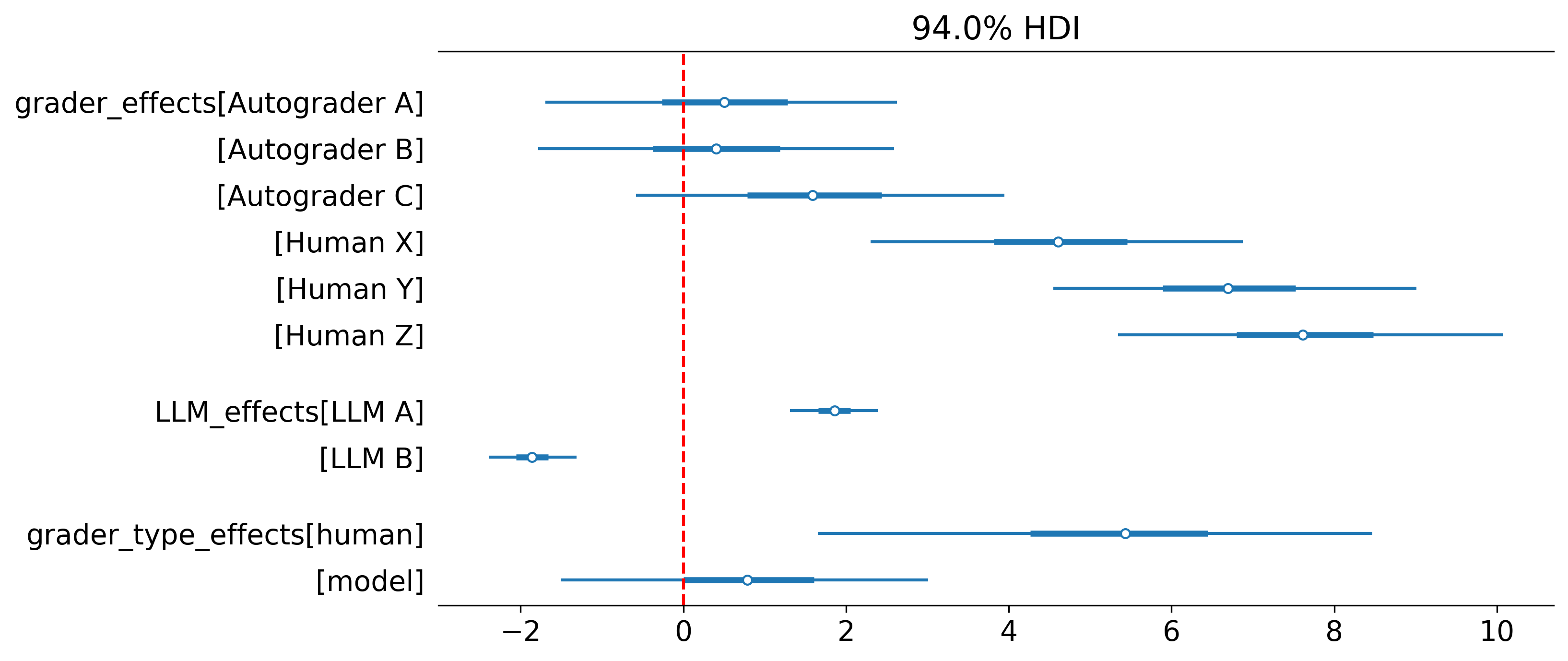
Question 3: Do autograders differ systematically from human experts?

To answer this question we can group the graders into human and LLM and utilise a hierarchicl GLM to reprent the group level effects (see the paper for a detailed explanation).

To achieve this we create a new variable which details the variable type using a custom processor.

data_process:
  path: ../custom_processors.py
  processors:
    - add_categorical_column: {new_column: grader_type, source_column: grader, mapping_rules: {Human: human}, default_value: model}
    - extract_observed_feature: {feature_name: score} # 0-10 rating
    - extract_features: {categorical_features: [grader, grader_type, LLM], effect_coding_for_main_effects: true, interactions: true}

1

specify the file where the custom processor is defined.

2

Calling the custom processor defined below.

@process
def add_categorical_column(
    new_column: str,
    source_column: str,
    mapping_rules: Dict[str, str],
    default_value: str = "unknown",
    case_sensitive: bool = False,
) -> DataProcessor:
    """
    Add a new categorical column to the processed data based on mapping rules (does the value contain the pattern).
    """

    def processor(
        state: AnalysisState, display: ModellingDisplay | None = None
    ) -> AnalysisState:
        def categorize(value):
            str_value = str(value)
            if not case_sensitive:
                str_value = str_value.lower()

            for pattern, category in mapping_rules.items():
                search_pattern = pattern if case_sensitive else pattern.lower()
                if search_pattern in str_value:
                    return category
            return default_value

        state.processed_data[new_column] = state.processed_data[source_column].apply(
            categorize
        )
        return state

    return processor

Check out how we defined a custom hierarchical model where grader effects inherit a group effect e.g. Human A inherits from the Human parameter in examples/skewed_score/custom_model.py.

The hierarchical model is a better fit to the data than the flat model.

Here we see a significant difference between human and LLM graders

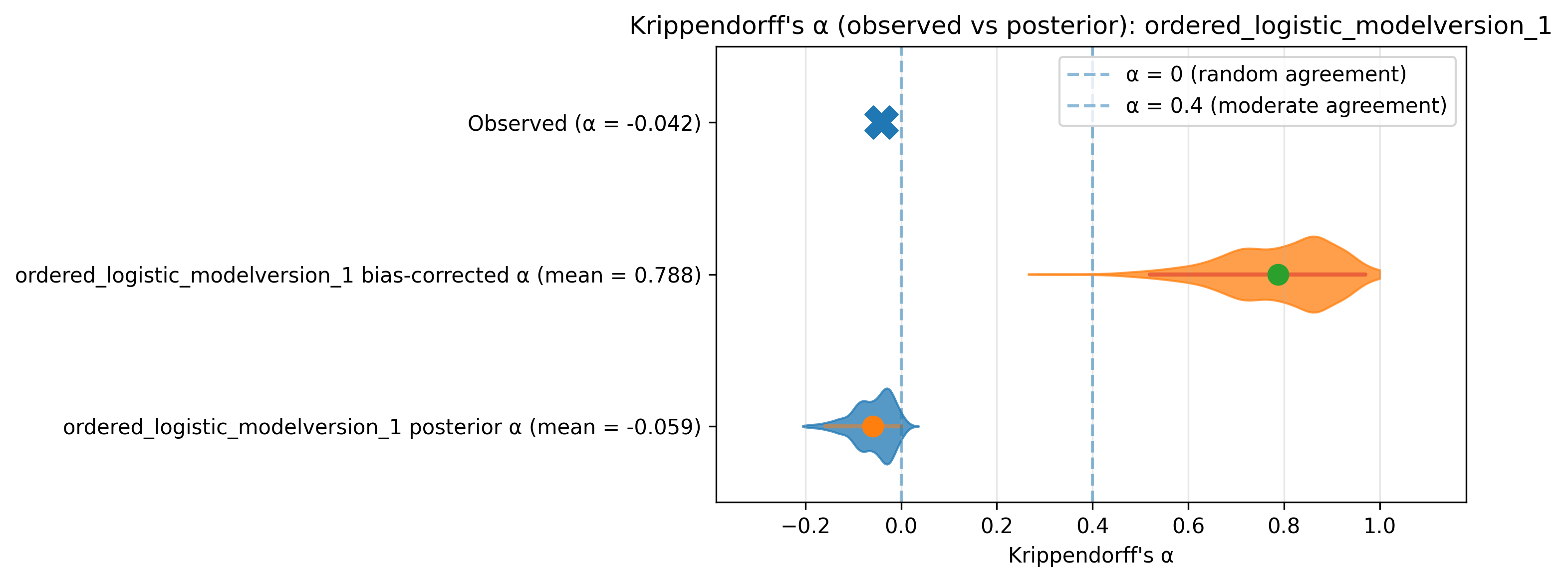
Question 4: How do scores differ at an item level?

To what extent do graders agree with one another? We can calculate Krippendorff’s alpha over simulated scores by sampling from the fitted GLM. This sounds quite complicated but can be easily implemented as a communicator!

@communicate
def krippendorff_alpha(
    *,
    max_draws_per_model: int = 1000,
    ci_level: float = 0.95,
    figsize: tuple[int, int] = (10, 4),
    title_prefix: str = "Krippendorff's α (observed vs posterior): ",
) -> Communicator:
    """
    Compute observed α and per-model posterior α distributions, and plot a separate
    figure for each model.
    """

    def communicate(
        state: AnalysisState,
        display: ModellingDisplay | None = None,
    ) -> Tuple[AnalysisState, CommunicateResult]:
        # Observed / "classical" α from raw data (shared across figs)
        classical_alpha = compute_krippendorff(state.processed_data)

        for model_analysis in state.models:
            if not model_analysis.is_fitted:
                continue

            if not model_analysis.inference_data.get("posterior_predictive"):
                if display:
                    display.logger.warning(
                        f"No posterior predictive samples for model {model_analysis.model_name} - skipping Krippendorff's alpha for this model. "
                        "If you want this, run with posterior predictive sampling enabled."
                    )
                continue

            # get alpha from posterior draws
            pred = (
                model_analysis.inference_data.posterior_predictive.obs.values
            )  # (chain, draw, N) <1>
            draws_flat = pred.reshape(-1, pred.shape[-1])  # (chain*draw, N)

            # Subsample draws for speed/reasonable CI
            rng = np.random.default_rng(0)
            take = min(max_draws_per_model, draws_flat.shape[0])
            idx = rng.choice(draws_flat.shape[0], size=take, replace=False)

            alphas = []
            for i in idx:
                df_i = state.processed_data[["grader", "item"]].copy()
                df_i["score_pred"] = draws_flat[i]
                a = compute_krippendorff(df_i, values_col="score_pred")
                if np.isfinite(a):
                    alphas.append(float(a))
            alphas = np.asarray(alphas, dtype=float)

            # counterfactual calculation omitted for brevity.


        return state, "pass"

    return communicate

2

Calculate alpha for each one of these draws. You can report the distribution of these alphas.

Output from the custom communicator. Here we compare between the classical method for computing Krippendorf’s alpha, how you can sample from fitted models and calculate arbitrary metrics over the sample distributions and finally how you can counterfactually intervene and finally, how to modify GLM parameters to remove systematic bias (orange plot) and answer other questions (please refer to the paper for more details)

Question 5: Do autograders favour longer outputs?

Until now we have focussed on categorical effects. GLMs of course can support continous parameters, often referred to as slopes. Here we add a slope investigating whether the length of response systematically affects LLM grader scores.

data_process:
  processors:
    - extract_observed_feature: {feature_name: first_is_chosen} # binary outcome
    - extract_features: {categorical_features: ['llm_pair', 'grader'], effect_coding_for_main_effects: true, interactions: true, continuous_features: [length_diff], standardise: true}

model:
  path: ../custom_model.py
  models:
    - name: pairwise_logistic_model
      config:
        tag: with_length_diff
        main_effects: ['llm_pair', 'grader', 'length_diff']
        effect_coding_for_main_effects: true
    - name: pairwise_logistic_model
      config:
        tag: without_length_diff
        main_effects: ['llm_pair', 'grader']
        effect_coding_for_main_effects: true

Adding the slope results in a better description of the data (using held one out validation).

For Autograders a longer response correlates with a significantly higher score!)